Strategy ONE
Lag
The Lag function is useful to display a set of metric values in an order determined by another metric or attribute on the report. This allows you to compare metric values side-by-side. The easiest way to understand the Lag function is with an example, provided below.
Syntax
Lag <BreakBy, SortBy> (Argument, Offset, DefaultValue)
Where:
BreakByis the attribute indicating where the calculation restarts.SortByis the attribute or metric by which the data is sorted.Argumentis an attribute or metric representing a list of values. It is common to use a metric forArgument.Offsetspecifies the offset from the current row to display information for. This offset trails behind the current row (you can use theLeadfunction to use an offset that precedes ahead of the current row, see Lead). For example, with an offset of two, row three displays data for the row two behind it, which would be row one.DefaultValueis the value displayed for any entries that do not have any data due to the offset. For example, when using an offset of 2, the first two entries use the default value.Some common default values to display include:
- 0: To display a value of 0 for any entries that do not have any data due to the offset, type
0. - No data: To display no data for any entries that do not have any data due to the offset, type
ZeroToNull(0).
- 0: To display a value of 0 for any entries that do not have any data due to the offset, type
Example
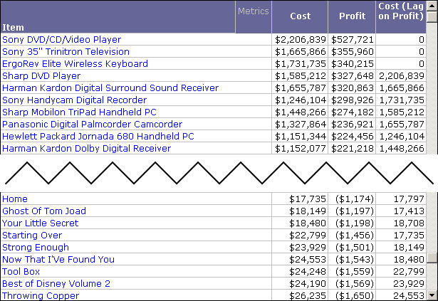
On a report with Item, Cost, and Profit, you can use the Lag function to create a Cost (Lag on Profit) metric. This metric displays Cost values based on the descending sort order of the Profit metric, and is defined with the following expression:
Lag<SortBy= (Profit Desc) >(Cost, 3.0, 0.0)
Notice that the offset is set to three, meaning that the display of cost values lags behind by three entries. This is displayed in the report results shown below.
Only the top and the bottom of the report is shown. To view the entire report results, you can create this report in the MicroStrategy Tutorial project.

The Cost (Lag on Profit) values are displayed three behind the Cost metric, and are displayed based on the descending sort order of Profit. Notice that with an offset of three, the first three entries for Cost (Lag on Profit) use the default value of zero. Also, the last three values of Cost are not included in the Cost (Lag on Profit) metric.
The report has been sorted based on the Profit metric to make the Cost (Lag on Profit) values easier to analyze.
Transformation-Style Analysis Using the Lag and Lead Functions
Transformation-style analysis can be supported using the Lag and Lead functions provided with MicroStrategy. These functions can be used to define metrics that compare values from different time periods without the use of transformations. For information on creating transformations, see the Project Design Guide.
- The examples shown below were created in the MicroStrategy Tutorial project.
-
The examples below use the
Lagfunction. TheLeadfunction can be used in the same way. The difference in usingLeadrather thanLagis that theLeadfunction would display information by going forward in time rather than backward. For example, while theLagfunction can return historical data from one year ago, the same formula used for theLeadfunction would return historical data from one year ahead.The
Leadfunction does not predict future values. For functions that can predict future values based on historical data, see ForecastV (Forecast, Vector Input), GrowthV (Growth, Vector Input), and TrendV (Trend, Vector Input). Additionally, you can use data mining functions from MicroStrategy Data Mining Services to predict future trends, as described in Data Mining Functions.
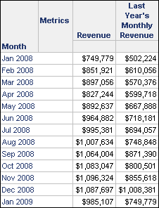
For example, a Last Year's Monthly Revenue metric can be created using the following function:
Lag<SortBy=(Month@ID)>(Revenue,12,ZeroToNull(0))
This metric can then be included on a report with the Month attribute and the Revenue metric, as shown below.

This allows you to perform a side-by-side comparison of monthly revenue for different years. In this report, the 2007 monthly revenue is displayed next to the 2008 monthly revenue. The element Jan 2009 is included to show that the Last Year's Monthly Revenue is displaying the monthly revenue from the previous year.
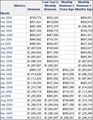
By modifying the offset of the Lag function, you can change the time periods that can be compared side by side. For example, the function listed above uses an offset of 12, which displays monthly data from one year ago. Using an offset of 3 would display monthly data from three months ago, while using an offset of 24 would display monthly data from two years ago. These slight modifications could be used to create separate metrics that could all be included on the same report. The report below shows an example of including three different metrics that use the same Lag formula with a different offset.

The report shown above allows side-by-side comparison of monthly revenue for three different time periods. In this report, the Monthly Revenue 2 Years Ago metric displays no data for months in the year 2008 because no revenue data exists for the year 2006.
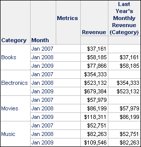
To use the Lag or Lead functions for transformation-style analysis, the metric formulas must be created to support the required reporting scenario. For example, the report with the Month attribute and the Revenue metric has the Category attribute added to it. To support this reporting scenario, you can modify the Lag formula described above to include the Category attribute, as shown below.
Lag<BreakBy={Category},SortBy=(Month@ID)> (Revenue,12,ZeroToNull(0))
Using the formula shown above, the calculation is restarted for each category, which allows the side-by-side comparison of monthly revenue over time for each category, as shown in the report below:

Only the Month attribute elements Jan 2007, Jan 2008, and Jan 2009 are displayed to show that the Last Year's Monthly Revenue (Category) metric is displaying the monthly revenue from the previous year.
