Creating a Predictive Model Using MicroStrategy

MicroStrategy Data Mining Services has been evolving to include more data mining algorithms and functionality. One key feature is MicroStrategy Developer's Training Metric Wizard. The Training Metric Wizard can be used to create several different types of predictive models including linear and exponential regression, logistic regression, decision tree, cluster, time series, and association rules.

Linear and Exponential Regression

The linear regression data mining technique should be familiar to you if you have ever tried to extrapolate or interpolate data, tried to find the line that best fits a series of data points, or used Microsoft Excel's LINEST or LOGEST functions.

Regression analyzes the relationship between several predictive inputs, or independent variables, and a dependent variable that is to be predicted. Regression finds the line that best fits the data, with a minimum of error.

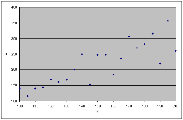
For example, you have a dataset report with just two variables, X and Y, which are plotted as in the following chart:

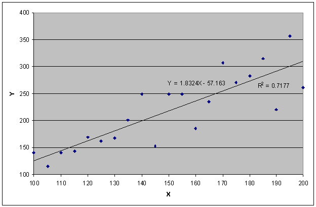
Using the regression technique, it is relatively simple to find the straight line that best fits this data, as shown below. The line is represented by a linear equation in the classic y = mx + b format, where m is the slope and b is the y-intercept.

Alternatively, you can also fit an exponential line through this data, as shown in the following chart. This line has an equation in the y = b mx format.

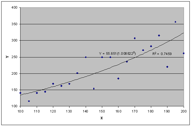
So, how can you tell which line has the better fit? Many statistics are used in the regression technique. One basic statistic is an indicator of the goodness-of-fit, meaning how well the line fits the relationship among the variables. This is also called the Coefficient of Determination, whose symbol is R2. The higher that R2 is, the better the fit. The linear predictor has an R2 of 0.7177 and the exponential predictor has an R2 of 0.7459; therefore, the exponential predictor is a better fit statistically.

With just one independent variable, this example is considered a univariate regression model. In reality, the regression technique can work with any number of independent variables, but with only one dependent variable. While the multivariate regression models are not as easy to visualize as the univariate model, the technique does generate statistics so you can determine the goodness-of-fit.

Logistic Regression

Logistic regression is a classification technique used to determine the most likely outcome from a set of finite values. The term logistic comes from the logit function, shown below:

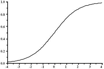
Notice how this function tends to push values to zero or one; the more negative the x-axis value becomes, the logit function approaches a value of zero; the more positive the x-axis value becomes, it approaches a value of one. This is how regression, a technique originally used to calculate results across a wide range of values, can be used to calculate a finite number of possible outcomes.

The technique determines the probability that each outcome will occur. A regression equation is created for each outcome and comparisons are made to select a prediction based on the outcome with the highest likelihood.

Evaluating Logistic Regression Using a Confusion Matrix

As with other categorical predictors, the success of a logistic regression model can be evaluated using a confusion matrix. The confusion matrix highlights the instances of true positives, true negatives, false positives, and false negatives. For example, a model is used to predict the risk of heart disease as Low, Medium, or High. The confusion matrix would be generated as follows:

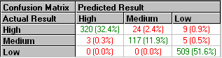
Proper analysis of the matrix depends on the predictive situation. In the scenario concerning heart disease risk, outcomes with higher false positives for Medium and High Risk are favored over increased false negatives of High Risk. A false positive in this case encourages preventative measures, whereas a false negative implies good health when, in fact, significant concern exists.

Cluster Analysis

Cluster analysis offers a method of grouping data values based on similarities within the data. This technique segments different items into groups depending on the degree of association between items. The degree of association between two objects is maximal if they belong to the same group and minimal otherwise. A specified or determined number of groups, or clusters, is formed, allowing each data value to then be mathematically categorized into the appropriate cluster.

Cluster analysis is seen as an unguided learning technique since there is no target or dependent variable. There are usually underlying features that determine why certain things appear related and others unrelated. Analyzing clusters of related elements can yield meaningful insight into how various elements of a dataset report relate to each other.

MicroStrategy employs the k-Means algorithm for determining clusters. Using this technique, clusters are defined by a center in multidimensional space. The dimensions of this space are determined by the independent variables that characterize each item. Continuous variables are normalized to the range of zero to one (so that no variable dominates). Categorical variables are replaced with a binary indicator variable for each category (1 = an item is in that category, 0 = an item is not). In this fashion, each variable spans a similar range and represents a dimension in this space.

The user specifies the number of clusters, k, and the algorithm determines the coordinates of the center of each cluster.

In MicroStrategy, the number of clusters to be generated from a set of data can be specified by the user or determined by the software. If determined by the software, the number of clusters is based on multiple iterations to reveal the optimal grouping. A maximum is set by the user to limit the number of clusters determined by the software.

The table below shows the result of a model that determines which of five clusters a customer belongs to.

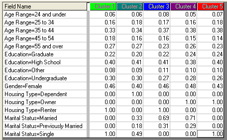
The center of each cluster is represented in the five cluster columns. With this information, it is possible to learn what the model says about each cluster. For example, since the center of Cluster 1 is where "Marital Status = Single" is one and all other marital statuses are zero, single people tend to be in this cluster. On the other hand, there is not a lot of variability across the clusters for the Age Range dimensions, so age is not a significant factor for segmentation.

Creating a cluster model is the first step, because while the algorithm will always generate the proper clusters, it is up to the user to understand how each cluster differs from the others.

Decision Tree Analysis

Decision trees are one of the most intuitive types of data mining model since they display an "if-then-else" structure that even the most novice user can understand. A decision tree is simple to follow and allows for very sophisticated analysis.

Decision trees separate a given dataset report into distinct subsets. Rather than employing the unguided learning approach used in cluster analysis (see Cluster Analysis), decision tree analysis uses a guided algorithm to create these subsets. The subsets share a particular target characteristic, which is provided by the dependent variable. Independent variables provide the other characteristics, which are used to divide the original set of data into subsets. Typically, the independent variable with the most predictive power is used first, then the next most powerful, and so on. MicroStrategy implements the Classification And Regression Tree (CART) algorithm to construct decision trees.

The image below displays a basic decision tree that includes its root node at the top. The connected nodes of the decision tree are traversed from top-to-bottom primarily and then left-to-right. Processing typically ends at the first leaf node (a leaf node is a node with no children) encountered with a predicate that evaluates to True.

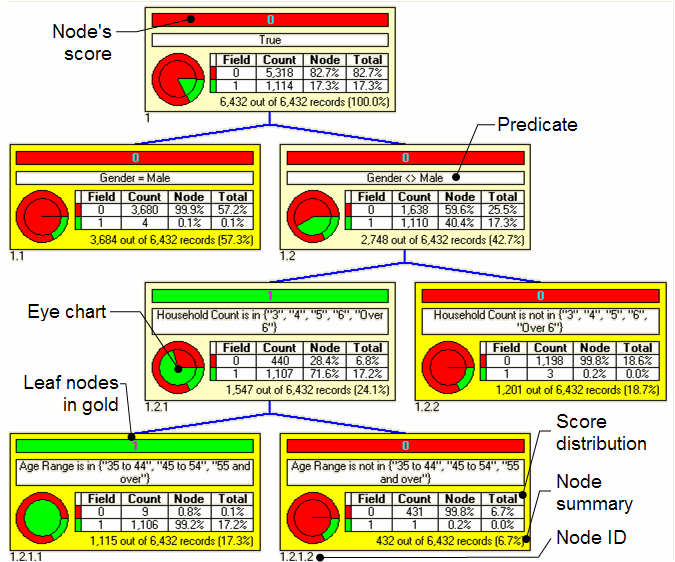
Each node includes the following information:

• Score: The most common (or dominant) result of the data records for the node.
• Predicate: A logical statement that is used to separate data records from a node's parent. Data records can belong to a node if the predicate evaluates to True. Predicates can be a single logic statement or a combination of multiple logic statements using operators such as AND, OR, XOR, and so on.
• Eye chart: A graphical representation of the distribution of scores, which is only shown if the PMML contains score distribution information. The outer ring chart shows the distribution of scores for all the data records in the training dataset report. The inner pie chart shows the distribution of scores for the data records in this node. The largest slice of the inner pie chart is the score for this node.
• Score distribution: A table showing the breakdown of training data records associated with the node, which serves also as the legend for the eye chart. The score distribution contains the actual count of training data records in this node, represented by each target class. The proportion of each class of data records is displayed as a percentage of the total counts for this node as well as a percentage of the total population. The node percentage for the dominant score can be considered as the confidence in the node's score. Score distributions are not required by PMML and, if not present, this score distribution table cannot be shown.
• Node summary: Percentage of all the training data records associated with this node. This information is descriptive only (not used to predict results directly) and can only be shown if the PMML contains score distribution information.
• Node ID: A reference for the node. MicroStrategy uses a level-depth format where the ID is a series of numbers representing the left-based position for each level.

The PMML specification for decision trees includes strategies for missing value handling, no true child handling, weighted confidences, and other features. For more details on these strategies, see the Data Mining Group website.

Association Rules Analysis

Association rules look for relationships between items. The most common example of this is market basket analysis.

Market basket analysis studies retail purchases to determine which items tend to appear together in individual transactions. Retailers use market basket analysis for their commercial websites to suggest additional items to purchase before a customer completes their order. These recommendations are based on what other items are typically purchased together with the items already in the customer's order. Market basket analysis provides the valuable ability to upsell a customer at the time of purchase, which has become a key requirement for any retailer.

The key to this type of analysis is the ability to find associations amongst the items in each transaction. This can include associations such as which items appear together the most frequently, and which items tend to increase the likelihood that other items will appear in the same transaction.

For example, five transactions from a grocery store are shown in the image below.

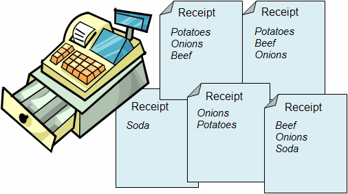
These transactions are summarized in the table below:

A 1 denotes that the item is included in the transaction, while a 0 denotes that the item is not included in the transaction.

Transaction ID	Soda	Potatoes	Onions	Beef
1	1	0	0	0
2	0	1	1	1
3	0	1	1	0
4	1	0	1	1
5	0	1	1	1

By reviewing the transaction table above, you can determine that beef appears in three out of the five transactions. In other words, 60% of all transactions support the item beef.

Support is a key concept that describes the relative frequency of transactions that contain an item or set of items, called an itemset. Itemset is another key concept in association rules since you can calculate associations not only for individual items but also between groups of items.

The table below shows the support for all possible combinations of one, two or three items per itemset (in other words, a maximum of three items per itemset).

Itemset	Transaction Count	Support
Beef	3	60%
Onions	4	80%
Potatoes	3	60%
Soda	2	40%
Beef, Onions	3	60%
Beef, Potatoes	2	40%
Onions, Potatoes	3	60%
Beef, Soda	1	20%
Onions, Soda	1	20%
Potatoes, Soda	0	0%
Beef, Onions, Potatoes	2	40%
Beef, Onions, Soda	1	20%
Beef, Potatoes, Soda	0	0%
Onions, Potatoes, Soda	0	0%

With this information, you can define rules that describe the associations between items or itemsets. The rules can be described as: The antecedent itemset implies the consequent itemset. In other words, the antecedent is a combination of items that are analyzed to determine what other items might be associated with this combination. These implied items are the consequent of the analysis.

For example, consider the rule Potatoes and Onions itemset implies Beef. This rule describes how transactions containing both potatoes and onions are related to those transactions that also contain beef. An association rule contains this qualitative statement but it is also quantified with additional statistics.

From the transaction table, you can determine that three out of five transactions contain the itemset potatoes and onions (antecedent), and two out of five transactions contain both the antecedent and the consequent. In other words, two out of three of the transactions containing potatoes and onions also contain beef.

Each association rule contains a confidence statistic that estimates the probability of a transaction having the consequent given the antecedent. In this example, after analyzing the five transactions, the confidence in this rule Potatoes and Onions itemset implies Beef is 67%. Confidence is calculated as follows:

Therefore, if a customer purchases both potatoes and onions, you can be 67% confident that beef would also be purchased, based on the five transactions analyzed.

By analyzing all combinations of these itemsets, an association rules model contains rules that describe the relationships between itemsets in a given set of transactions. The table below shows the confidence in all the rules found in this example scenario.

	Consequent
Antecedent	Beef	Onions	Potatoes	Soda
Beef		100%	67%	33%
Onions	75%		75%	25%
Potatoes	67%	100%		0%
Soda	50%	50%	0%
Beef, Onions			67%	33%
Beef, Potatoes				0%
Onions, Potatoes	67%			0%
Beef, Soda
Onions, Soda	100%

This model contains 22 different rules based on only four different items and five transactions. Since a typical retailer can have thousands of items and potentially millions of transactions, this type of analysis can generate a large number of rules. It is typical that the vast majority of these rules will have a low confidence (notice in the table above that the lowest confidences are rules that have a consequent containing soda).

In order to limit the volume of rules generated, you can control:

• Maximum number of items per antecedent: This setting defines the maximum number of items that can be included in each antecedent itemset (consequent itemsets can only contain a single item). For example, if set to three, items for each antecedent will be grouped into itemsets containing one, two, or three items. In the example above that includes the four items beef, onions, potatoes, and soda, a maximum of two creates antecedents with no more than two items, while still including each item in the analysis.
• Minimum confidence: The minimum probability that qualifying rules should have. For example, if set to 10%, then an association rule must have a confidence of 10% or more to appear in the model.
• Minimum support: The minimum number of transactions an itemset must occur in to be considered for an association rule. For example, if set to 1%, then itemsets must appear, on average, in one transaction out of 100.
• Maximum consequent support: The maximum support of the consequent allowed for qualifying rules. This can be used to avoid including obvious recommendations in the resulting rules. For example, if set to 99%, then rules that have a consequent support greater than 99% are not included in the resulting model.

In addition to support and confidence, association rules can also include the following statistics:

• Lift: Lift is a ratio that describes whether the rule is more or less significant than what one would expect from random chance. Lift values greater than 1.0 indicate that transactions containing the antecedent tend to contain the consequent more often than transactions that do not contain the antecedent. The table below shows the lift of the rules in our example model. Note that onions are an above average predictor of the purchase of beef and potatoes.

  	Consequent
  Antecedent	Beef	Onions	Potatoes	Soda
  Beef		1.25	1.11	0.83
  Onions	1.25		1.25	0.63
  Potatoes	1.11	1.25		0.00
  Soda	0.83	0.63	0.00
  Beef, Onions			1.11	0.83
  Beef, Potatoes				0.00
  Onions, Potatoes	1.11			0.00
  Beef, Soda
  Onions, Soda	1.67

• Leverage: Leverage is a value that describes the support of the combination of the antecedent and the consequent as compared to their individual support. Leverage can range from -0.25 to 0.25, and a high leverage indicates that there is a relationship between the antecedent and the consequent. For example, if 50% of the transactions contain the antecedent and 50% of the transactions contain the consequent, you would expect 25% of the transactions to contain both the antecedent and the consequent if they were completely independent; this would correspond to a leverage of zero. If more than 25% of the transactions contain the antecedent and consequent together, then there is a positive leverage (between 0 and 0.25). This positive leverage indicates that the antecedent and consequent appear more frequently than you would expect if they were completely independent, and can hint at a relationship.
• Affinity: Affinity is a measure of the similarity between the antecedent and consequent itemsets, which is referred to as the Jaccard Similarity in statistical analysis. Affinity can range from 0 to 1, with itemsets that are similar approaching the value of 1.

Time Series Analysis

Time series represents a broad and diverse set of analysis techniques which use a sequence of measurements to make forecasts based on the intrinsic nature of that data. While most other data mining techniques search for independent variables that have predictive power with respect to a particular dependent variable, time series analysis has just one variable. The past behavior of the target variable is used to predict its future behavior.

This past behavior is measured in a time-based sequence of data, and most often that sequence is a set of measurements taken at equal intervals in time. By analyzing how values change over time, time series analysis attempts to find a model that best fits the data.

There is also an implied assumption that the data has an internal structure that can be measured, such as level, trend, and seasonality.

Time series forecasts are only statistically valid for projections that are just one time period beyond the last known data point. The techniques used to determine the model parameters are focused on reducing the one-step-ahead error. Forecasts two or more steps ahead are less reliable since they go beyond the forecast horizon considered when the model was developed.

In time series analysis, many models are tested and each model is structured to match a certain data profile.

For example, consider this set of data:

Month	Target	Average	Three-Month Moving Average	Three-Month Centered Moving Average
1	170	293
2	200	293		200
3	230	293	200	233
4	270	293	233	250
5	250	293	250	263
6	270	293	263	277
7	310	293	277	303
8	330	293	303	317
9	310	293	317	330
10	350	293	330	343
11	370	293	343	390
12	450	293	390

The first two columns contain the data to be modeled. The target, which could be anything from sales revenue to units sold can be used to create a few simple models:

• The Average column is simply the average of all twelve data points.
• Each data point in the Three-Month Moving Average is the average of the previous three months target data. Since this model contains a series of subset averages, it does a better job of following the data than the simple average. But since it averages the past three months, it tends to lag behind the target data. The last value is at time t but it can never catch the upward trend of the target.
• The right most column is a centered version of the Three-Month Moving Average. Each data point in this column is an average of the prior, current, and next month. This is an improvement over the non-centered version since the lag has been eliminated, but at the cost of delaying the forecast. The last value is at time t-1 but it tracks the upward trend closely.

The differences between the three models becomes clear when the data is plotted on the chart shown below.

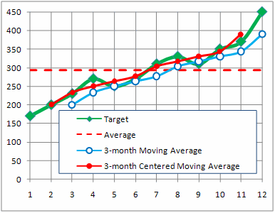
The Average model simply captures the level of the data. If our Target data was flat without a significant upward or downward trend, a simple average might make a sufficient model. But in this case, with the data trending strongly upward, it is not a good fit.

Both moving average models do a better job. The centered moving average avoids the lag problem by delaying its calculation and therefore is the best fit.

The technical definition of best fit is the model with the lowest Root Mean Square Error (RMSE). The RMSE is calculated by taking the square root of the average difference between the actual data and the forecast at each time period.

In all three models, the averages have the effect of smoothing the data by diminishing the peaks and valleys. The simple 12-month average is a constant and therefore completely smooth. On the other hand, the moving three-month averages still have some ups and downs, but not as strongly as the original target data. The challenge for finding the best model is determining the proper time horizon to forecast over. This is especially true when the data is not stationary but has a significant trend, since older values can hide more recent changes.

A common solution is a technique is called exponential smoothing. In order to understand how exponential smoothing works, it is helpful to see how the technique is derived from moving averages. The generic formula for calculating averages is:

One way of thinking of an average is that it is the sum of each value weighted by 1/n. Our simple 12-month average gave equal weight (one twelfth) to each month. The three-month moving averages gave each month a weight of one-third.

Exponential smoothing gives more recent values greater influence on the result. Older values are given exponentially decreasing weight. The generic exponential smoothing formula is:

Where:

• Si = Smoothed Observation

• = A smoothing constant, determines how quickly or slowly weights decrease as observations get older

  Over many observations, the smoothing effect follows an infinite series that approximates an exponential function.

In exponential smoothing, the algorithm determines the smoothing constant that results in the lowest RMSE for a given time series profile. The state of the art approach to exponential smoothing, described by Everette S. Gardner, attempts to find the best profile that matches the data used to train the model. In particular, each profile can be described by two aspects, trend and seasonality.

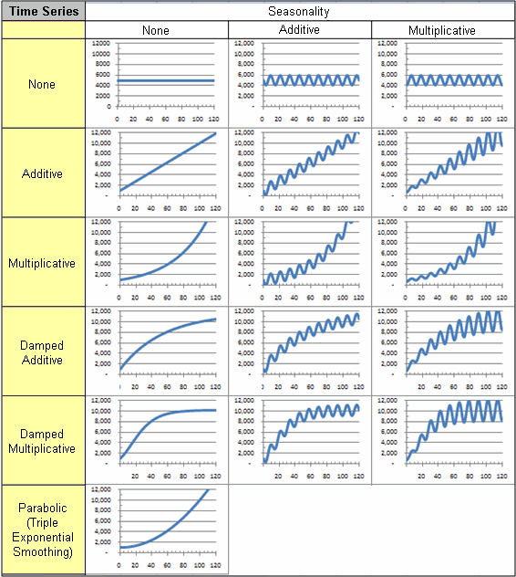
Trend is the dominant direction that the data is heading towards, as a function of time. Exponential Smoothing includes the following trend types:

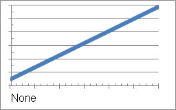
• None: This is the simplest case, in which there is no trend. This means that the data is not dominated by either an upward or a downward progression, as shown in the example below:

  

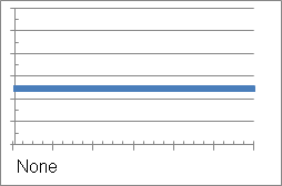
  The following equation describes this trend line:

  

  Where is the value being forecast, and is a constant representing the level of the data.

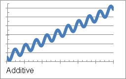
• Additive: An additive trend is evident when the time series data changes an equal amount per time period, as shown in the example below:

  

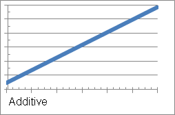
  The following equation describes this trend line:

  

  Where is the value being forecast, is the level, is slope or constant trend, and t is the number of periods ahead of the last known data point in the time series.

• Damped additive: With this trend, the amount of change decreases each successive time period. This can help to reflect most real world systems and processes, in which a trend is constrained from progressing indefinitely without change.

  The rate of this damping is governed by the damping parameter (phi). The value of phi can vary from zero to one, with the damping effect becoming smaller as phi approaches one.

  The additive trend is the same as a damped additive trend with .

  The value of phi is the one that results in the lowest RMSE. This trend is shown in the following example:

  

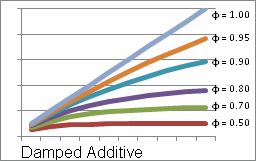
  The following equation describes this trend line:

  

  Where is the value being forecast, is the level, is slope or constant trend, and t is the number of periods ahead of the last known data point in the time series. The damping is calculated using the following formula:

  

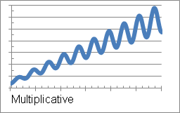
• Multiplicative: A multiplicative trend is one where the trend is not constant, but the trend changes at a fixed rate, as shown in the example below:

  

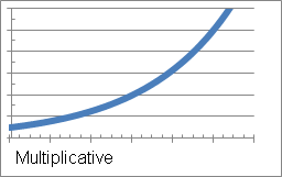
  The following equation describes this trend line:

  

  Where is the value being forecast, is the level, is slope or constant trend, and t is the number of periods ahead of the last known data point in the time series.

• Damped multiplicative: This trend is one where the rate of change in the trend decreases over time, subject to the damping parameter , as shown in the example below:

  

  The following equation describes this trend line:

  

  Where is the value being forecast, is the level, is the rate at which the undamped trend changes, and t is the number of periods ahead of the last known data point in the time series. The damping is calculated using the following formula:

  

• Triple exponential: This trend is evident when the time series data follows a parabolic profile, as shown in the example below:

  

  The following equation describes this trend line:

  

  Where is the value being forecast, is the level, is the slope or constant trend, is the rate of acceleration of the trend, and t is the number of periods ahead of the last known data point in the time series.

The other aspect that describes the time series profile is seasonality. Seasonality accounts for seasonal differences that appear in the time series data. When creating models with MicroStrategy using the Training Metric Wizard, the user defines the number of time periods in the seasonal cycle. For example, with monthly data you could define each month as its own season by using 12 as the value for the seasonality. Similarly, with quarterly data you could define each quarter as its own season by using four as the value for the seasonality.

Exponential Smoothing includes the following seasonality types:

• None: There are no seasonal factors in the time series, as shown in the example below:

  

  To use this type of seasonality, in the Training Metric Wizard, specify zero as the number of time periods for the seasonal cycle.

• Additive: Seasonal factors are added to the trend result. This means that each season's effect on the profile is constant, as shown in the example below:

  

  This profile is considered only when the number of time periods in the seasonal cycle, specified in the Training Metric Wizard, is two or more.

• Multiplicative: Seasonal factors are multiplied by the trend result. This means that seasonal effects increase as the trend of the data increases, as shown in the example below:

  

  This profile is considered only when the number of time periods in the seasonal cycle, specified in the Training Metric Wizard, is two or more.

By combining trend and seasonality, the following are all of the possible time series profiles:

Predictive Model Workflow

To create a predictive model, you must do the following, in order:

1. Create the training metrics using the Training Metric Wizard. For information, see Creating a Training Metric with the Training Metric Wizard.
2. Create a training report containing the training metric. This training report will generate the dataset used to train the predictive models.
3. Create the predictive metric from the training metric by executing the training report. For information, see Create Predictive Metrics from Training Metrics.
• Since Exponential Smoothing gives greater weight to more recent data, time series models should be updated whenever new data is available. While this can be said for other types of model as well, this is particularly true for time series models since recent results can significantly influence the model. Therefore, for time series models, it is common to deploy the training metrics instead of the predictive metrics. This guarantees the time series forecast results reflect the most recent data.
• If the option to automatically create predictive metrics is selected when the training metric is created, simply execute the training report. The predictive metric is generated according to the parameters of the training metric. You can now use the predictive metric on reports or other MicroStrategy objects. For information, see Using the Predictive Metric.
• If the option to automatically create predictive metrics is not selected when the training metric is created, execute the training report and then use the Create Predictive Metrics option. For steps, see To Use the Create Predictive Metrics Option in the Report Editor. You can then use the predictive metric, as discussed in Using the Predictive Metric.

Creating a Training Metric with the Training Metric Wizard

Recall that the Data Mining Services workflow develops a predictive model based on a dataset report. When you use MicroStrategy, this dataset report is generated in the form of a MicroStrategy report or MDX cube, with the basic format shown in the following report sample:

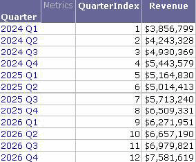
The dataset report shown above can be used to develop a predictive model to forecast on-line sales per quarter. The process of developing this predictive model is called training the model. Data Mining Services uses a particular type of metric called a training metric to develop the predictive model. When the training metric is added to the dataset report, it analyzes the data and generates a forecast, as shown below.

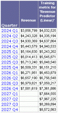
This training metric uses a powerful function that forecasts the results shown in the previous report, given the proper parameters. It also generates a predictive model that can be used to forecast future outcomes. The MicroStrategy Training Metric Wizard allows you to easily create training metrics.

To Create a Training Metric

1. In MicroStrategy Developer, you can create the following types of training metrics:
• Stand-alone training metric: Stand-alone training metrics exist in metadata and are the standard type of training metric that can be used on any report. You can use metrics and attributes within the project as inputs to create stand-alone training metrics.

  To create a stand-alone training metric, from the Tools menu, select Training Metric Wizard.

• Derived training metric: Derived training metrics are training metrics that are created using the derived metrics feature. You must have MicroStrategy OLAP Services to create derived metrics. Derived training metrics also have the same requirements and restrictions as derived metrics (see the In-memory Analytics Help). This capability is particularly useful during the exploratory phase of the data mining process, during which many different variables are tried in a variety of modeling configurations.

  Derived training metrics can be created directly on reports as well as reports that are added as Grid/Graphs on documents:

  • For standard reports, navigate to a report, right-click the report, and select Run. The Report Editor opens. From the Insert menu, select New Training Metric.
  • For reports that are added as Grid/Graphs on documents, right-click the Grid/Graph within the document and select Edit Grid. From the Insert menu, select New Training Metric.
• MDX cube training metrics: If you integrate MDX cube sources into MicroStrategy as MDX cubes, you can create training metrics based off of the MDX cube data. You can use metrics and attributes within the MDX cube as inputs to create MDX cube training metrics.

  Using either the MDX Cube Catalog or the MDX Cube Editor to view an imported MDX cube, choose Edit > Training Metric Wizard.

  The Introduction page of the Training Metric Wizard opens. To skip the Introduction page when creating training metrics in the future, select the Don't show this message next time check box.

2. Click Next to open the Select Type of Analysis page.
3. Select a type of analysis from the following:
• Linear regression: The function attempts to calculate the coefficients of a straight line that best fits the input data. The calculated formula has the following format:

  

  where y is the target variable and X1…Xn are the independent variables.

• Exponential regression: The function attempts to calculate the coefficients of an exponential curve that best fits the input data. The natural log (ln) of the input target variables is calculated and then the same calculations used for linear regression are performed. Once the straight-line coefficients are calculated, exponential regression uses the natural exponential of the values, which results in the coefficients for the formula of an exponential curve. The calculated formula has the following format:

  

  where y is the target variable and X1…Xn are the independent variables.

• Logistic regression: The function is used to determine the most likely outcome of a set of finite values. The technique uses a chi-square test to determine the probability of each possible value and provide a predicted outcome based on the highest likelihood.
• Cluster: This function offers a method of grouping data values based on similarities within the data. A specified or determined number of groups, or clusters, is formed allowing each data value to be mathematically categorized into the appropriate cluster.
• Decision tree: The function generates a series of conditions based on independent input to determine a predicted outcome. The result is a hierarchical structure with the ability to lead a set of input to the most likely outcome.
• Time Series: This function attempts to make forecasts based on a series of time-related input data. It consists of numerous techniques that can be applied to either seasonal or non-seasonal data.
• Association: This function looks for relationships between items. The most common example of this is market basket analysis.

4. Set specialized parameters based on the Type of Analysis selected:

   Analysis Type	Parameters
   Cluster	Do one of the following: Specify the exact number of clusters to be generated from the set of data. Allow MicroStrategy Data Mining Services to determine the optimal number of clusters based on the training data. The algorithm creates multiple models, starting with two clusters, and continues to add more clusters one at a time. With each additional cluster, the quality of the model is assessed. The quality of the current model is measured by calculating the total distance of all records to the centers of their assigned clusters (DCurr). This result is compared to the same result for the previously generated model (DPrev). This process continues until the amount of improvement, (DPrev – DCurr) / DPrev, is less than the amount specified by the percent improvement parameter, or the maximum number of clusters is reached. Upon completion of this process, the model with the best quality is used in the predictive metric.
   Decision tree	When MicroStrategy trains a decision tree model, the decision tree algorithm splits the training data into two sets; one set is used to develop the tree and the other set is used to validate it. Prior to MicroStrategy 9.0, one fifth of the training data was always reserved for validating the model built on the remaining four fifths of the data. The quality of this model (referred to as the holdout method) can vary depending on how the data is split, especially if there is an unintended bias between the training set and the validation set. Introduced in MicroStrategy 9.0, K-folds cross-validation is an improvement over the holdout method. The training data is divided into k subsets, and the holdout method is repeated k times. Each time, one of the k subsets is used as the test set and the other k-1 subsets are used to build a model. Then the result across all k trials is computed, typically resulting in a better model. Since every data point is in the validation set only once, and in the training dataset k-1 times, the model is much less sensitive to how the partition is made. A downside is that training time tends to increase proportionally with k, so MicroStrategy allows the user to control the k parameter, limiting it to a maximum value of 10.
   Time series	Number of time periods in the seasonal cycle: This value allows for the specification of seasonality inherent to the training data, and may be defined as follows: Zero (default) or 1: This indicates that no attempt is made during analysis to find seasonality in the training data. In this case, two types of analysis are performed: double (linear) and triple (quadratic) exponential smoothing. Once the analyses are complete, the model which best fits the training data is created. > 1: This indicates that the training data has seasonality, consisting of the specified number of time periods. In this case, two types of Winter's exponential smoothing (additive and multiplicative) are performed. Once the analyses are complete, the model which best fits the training data is created.
   Association	Maximum number of items per antecedent: This setting defines the maximum number of items that can be included in each antecedent itemset (consequent itemsets can only contain a single item). For example, if set to three, items for each antecedent will be grouped into itemsets containing one, two, or three items. In a transaction that includes the four items beef, onions, potatoes, and soda, a maximum of two creates antecedents with no more than two items, while still including each item in the analysis. The default value for this setting is two. Increasing this number may lead to the generation of more rules and, as a consequence, long execution time for training reports. Minimum confidence: The minimum probability that qualifying rules should have. For example, if set to 10%, then an association rule must have a confidence of 10% or more to appear in the model. The default value for this setting is 10%. Increasing this value may lead to the generation of fewer rules. Minimum support: The minimum number of transactions an itemset must occur in to be considered for an association rule. For example, if set to 1%, then itemsets must appear, on average, in one transaction out of 100. The default value for this setting is 10%. Increasing this value may lead to the generation of fewer rules. Maximum consequent support: The maximum support of the consequent allowed for qualifying rules. This can be used to avoid including obvious recommendations in the resulting rules. For example, if set to 99%, then rules that have a consequent support greater than 99% are not included in the resulting model. The default value for this setting is 100%. Decreasing this value may lead to the generation of fewer rules.

5. Click Next to open the Select Metrics page.
6. Select the metrics and attributes from your project or MDX cube to be used in the training metric. To locate and select the metrics and attributes to be used, you can use the following:
• Object Browser: This option is available for all types of training metrics. Use the Object Browser to browse your project for metrics and attributes to be used in the training metric. If you are creating MDX cube training metrics, you can only select metrics and attributes within the MDX cube.
• Report Objects: This option is available if you are creating derived training metrics only. Use the Report Objects to select attributes and metrics from the report to be used in the training metric.

7. To add a metric or attribute to use in the training metric, click the right arrow next to the type of metric. For example, to add a dependent metric, select the metric in the Object Browser, then click the right arrow next to Dependent Metric.

   If an attribute is selected as a input, the Training Metric Wizard automatically creates a metric expression to be used as input to the training metric. By default, this expression uses the following format:

   Max(AttributeName){~}

   The ID form of the attribute is used as an input to the training metric. If a different attribute form should be used as an input, a metric must be manually created prior to creating the training metric. For steps on how to create this metric, see Inputs for Predictive Metrics.

   The different metrics that make up the training metric are described below.

   • Dependent Metric is the metric or attribute representing the field value to be predicted by the model. All types of analysis except cluster analysis require a dependent metric.

     You can select only one dependent metric or attribute.

   • Independent Metrics are the metrics and attributes for each of the independent variables to be considered while generating the predictive model. All types of analysis require independent metrics or attributes.

     Select at least one independent metric or attribute.

   • Segmentation Metrics are optional selections that apply only to linear, exponential, and logistic regression analyses. The Training Metric Wizard can generate either regression models or tree regression models.
   • In a tree regression model, the leaves of the tree contain a regression model trained on the records associated with that leaf of the tree. For example, if a metric or attribute representing a geographic region is used as a Segmentation Metric, each region will have its own unique forecast. Thus, multiple regression models can be included in a single predictive metric.
   • Add one metric or attribute to represent each level within the tree of the model.
   • If no Segmentation Metrics are specified, a standard regression model is generated.
8. You can use the default options for the algorithm and variable settings by clearing the Show advanced options check box. To specify more options for these settings, do the following:
1. Select the Show advanced options check box.
2. Click Next to open the Advanced Options page.
3. You can define variable reduction for linear and exponential regression.
4. To specify options for independent and dependent inputs, click Advanced Variable Settings. See the online help for more information on these settings. To save your changes and return to the Advanced Options page, click OK.
9. Click Next to open the Select Output page.
10. Select the destination of where each predictive metric is saved. Your options depend on the type of training metric being created:
• Folder: This option is available if you are creating stand-alone training metrics or derived training metrics. Click ... (the Browse button) to define the location in your MicroStrategy project to save the predictive metrics created by the training metric. If you select this option, predictive metrics are saved as stand-alone predictive metrics.

  If you are using derived training metrics, you should select this option when a predictive model worthy of deployment is found. Selecting this option saves the predictive model as stand-alone predictive metrics.

• Report Objects: This option is available if you are creating derived training metrics only. Select this option to create the predictive metrics as derived predictive metrics. A derived predictive metric exists only within the report used to create the predictive metric. This capability is particularly useful during the exploratory phase of the data mining process, during which you can test many variables and create a large variety of models.

  The way in which derived predictive metrics are created depends on whether the derived training metrics are included directly on a report or on a report included in a document as a Grid/Graph:

  • When the report is executed to create predictive metrics (see Create Predictive Metrics from Training Metrics), the following occurs:
  • The derived training metrics are moved off the report's template; the template determines what is displayed for the report. The derived training metrics are still available in the Report Objects of the report, which supplies the definition of the report. If you update the derived training metrics and need to re-create their associated derived predictive metrics, you must add the derived training metrics back to the template of the report. When the derived predictive metrics are re-created, new versions are created to keep a history of the predictive modeling.
  • Any derived training metrics that are moved off the report's template during report execution are replaced with the first predictive metric selected to be generated for the derived training metric. When the derived training metric is initially replaced with the derived predictive metric, the values are not automatically updated to reflect the predictive metric analysis. Re-execute the report to update the values for the derived predictive metric.
  • All other predictive metrics selected to be generated are added to the Report Objects and are not on the report grid by default. This makes the predictive model available for viewing only. To execute the derived predictive metric, you must add the derived predictive metric to the grid of the report.
  • When the document including the report as a Grid/Graph is executed to create predictive metrics (see Create Predictive Metrics from Training Metrics), the following occurs:
  • All predictive metrics are added to the available dataset objects for the report and are not included on the report grid by default. These predictive metrics are not saved in the report itself and are only available with the report as a dataset in the current document. This makes the predictive model available for viewing only. To execute the derived predictive metrics, you must add the derived predictive metrics to the grid of the report or directly to a section within the document.
  • Managed Objects folder: If you are creating MDX cube training metrics, the training metrics are created in the Managed Objects folder of the MicroStrategy project.
11. To automatically create the predictive metric each time a report that contains the training metric is executed, select the Automatically create on report execution check box. This option automatically overwrites any predictive metrics saved with the same name in the specified location. If you do not want to overwrite the predictive metric, clear this check box. For more information, see Create Predictive Metrics from Training Metrics.

    If you are creating a derived training metric, the Automatically create on report execution check box is selected and cannot be cleared. This is to ensure that predictive metrics can be created for the derived training metric, since derived training metrics are only available as part of a report or document.

12. To include verification records within the model, specify the number of records to include.

    If the number of records is set to zero, model verification is not included in the model.

    Model verification records are used by the consumer of the model to insure that the results of the consumer are equal to the results intended by the model producer. Each record contains a row of input from the training data along with the expected predicted output from the model.

13. If you are performing Association rules analysis, click Rules. The Rules to Return dialog box opens.

    These criteria determine which rules will be returned as output for a particular input itemset. You can choose from the following options:

    • Rule selection criteria:
    • Antecedent only (Recommendation): Select rules when the input itemset includes the antecedent itemset only. This is the default behavior. Its purpose is to provide a recommendation, based on the input itemset.
    • Antecedent and consequent (Rule matching): Select rules when the input itemset includes both the antecedent and consequent itemsets. Its purpose is to locate rules that match the input itemset.
    • Return the top ranked rules: These options allow for the specification of exactly which rule is to be returned, based on its ranking among all selected rules.
    • Return the top ranked rules up to this amount: Defines the maximum number of rules that are to be returned. For instance, if set to three, the top three rules can be returned as output. In this case, three separate predictive metrics are created. The default value for this setting is one, and its maximum value is 10.
    • Rank selected rules by: Defines whether the rules are be ranked by confidence, support, or lift. Multiple selections may be specified.
    • Select all rules (One rule per row): This option allows for the creation of a report which displays all rules found within the model. If the corresponding predictive metric is placed on a report, a single rule is returned for each row of the report. The rules are returned in the order they appear within the model, and are not based on an input itemset.
14. Select the Predictive Metric(s) to generate.
• A training metric can produce different output models when it is run on a training report. You must select at least one output model so that the training metric is created, although you can select multiple outputs. A predictive metric will be generated for each output.

  For example, if Predicted Value and Probability are selected as output models, then two predictive metrics will be created during the training process. One will output the predicted outcome when used on a report while the other will output the probability of the predicted outcome.

  If no predictor type is selected, Predicted Value is selected automatically.

• A default aggregation function is displayed for all types of predictive metrics. The default is the recommended function based on the type of values produced by each model. The aggregation function ensures proper results when drilling and aggregating from a MicroStrategy report.

  If desired, you can change the aggregation functions by using the drop-down lists of functions.

  If non-leaf level metrics from different hierarchies are used as independent metrics and tree level metrics, you may want to set the aggregation function to None. This can avoid unnecessary calculations and performance degradation. For example, the Quarter attribute from the Time hierarchy is used as an independent variable and Region from the Geography hierarchy is used as a tree level metric. Multiple calculations for each quarter's region can result.

15. Click Next. The Summary page opens.
16. Click Finish. If it is a derived training metric, the derived training metric is saved in the report with a default name. Otherwise, the Save As dialog box opens.
17. Select the MicroStrategy project folder in which to save the new metric. MDX cube training metrics must be saved in the Managed Objects folder of the MicroStrategy project.
18. Enter a name for the new metric.
19. Click Save.

Create Predictive Metrics from Training Metrics

You can quickly and easily create predictive metrics from training metrics in either of the following ways:

• If the option to automatically create predictive metrics is disabled on the training metric, execute the training report and then use the Create Predictive Metrics option. For steps, see To Use the Create Predictive Metrics Option in the Report Editor.

  The Create Predictive Metrics option is available only when you are running reports in MicroStrategy Developer.

• If the option to automatically create predictive metrics is enabled on the training metric, execute the training report to create the predictive metric. This is the default behavior, and is controlled by the Automatically create on report execution check box described in Creating a Training Metric with the Training Metric Wizard.

  If you are using derived predictive metrics and have selected to save the derived predictive metrics to the Report Objects, these derived predictive metrics are created in the following ways:

  • When a report is executed to create predictive metrics, the following occurs:
  • The derived training metrics are moved off the report's template; the template determines what is displayed for the report. The derived training metrics are still available in the Report Objects of the report, which supplies the definition of the report. If you update the derived training metrics and need to re-create their associated derived predictive metrics, you must add the derived training metrics back to the template of the report. When the derived predictive metrics are re-created, new versions are created to keep a history of the predictive modeling.
  • Any derived training metrics that are moved off the report's template during report execution are replaced with the first predictive metric selected to be generated for the derived training metric. When the derived training metric is initially replaced with the derived predictive metric, the values are not automatically updated to reflect the predictive metric analysis. Re-execute the report to update the values for the derived predictive metric.
  • All other predictive metrics selected to be generated are added to the Report Objects and are not on the report grid by default. This makes the predictive model available for viewing only. To execute the derived predictive metric, you must add the derived predictive metric to the grid of the report.
  • When a document including the report as a Grid/Graph is executed to create predictive metrics, the following occurs:
  • All predictive metrics are added to the available dataset objects for the report and are not included on the report grid by default. These predictive metrics are not saved in the report itself and are only available with the report as a dataset in the current document. This makes the predictive model available for viewing only. To execute the derived predictive metrics, you must add the derived predictive metrics to the grid of the report or directly to a section within the document.

After the predictive metric is created in any of these ways, you can use it in reports, documents, and other objects, as discussed in Using the Predictive Metric.

To Use the Create Predictive Metrics Option in the Report Editor

1. Using MicroStrategy Developer, add the training metric to a report.

   Ensure that the training metric is on the grid of the report. If the training metric is only in the Report Objects but not on the report grid, no predictive metrics are created for the training metric when the report is executed.

2. Execute the training report in MicroStrategy Developer.

   The Create Predictive Metrics option is available only when you are running reports in MicroStrategy Developer.

3. Choose Data > Create Predictive Metric(s). The Create Predictive Metric(s) dialog box opens.
4. To view information about a training metric, select it from the Metrics list.
5. To temporarily rename the predictive metric created by the selected training metric, enter the new name in the Name box.

   The new name is generated when you click OK, but the changes are not saved when the report is closed.

6. You can change the options and associated aggregation function for producing the predictive metric in the Aggregation function area.

   The new options are applied when you click OK, but the changes are not saved when the report is closed.

7. To save the PMML from the generated model, click Generate PMML File and select a location in which to save the PMML file.
8. Click OK.

   The predictive metric is created in the location specified by the training metric. It is generated according to the parameters of the training metric.